An EM algorithm for a Mixture of Gamma distributions in Python
Introduction
I recently came across mixture models in a soft clustering task for my work and the first thing that came to my mind was Gaussian Mixture Models (GMM). There are many tutorials, a scikit-learn class and a lot of resources on the internet about it. So I tried it… and I quickly noticed that is was not well suited to fit my data.
Why Gaussian Mixtures sometimes fail?
A Gaussian component assumes:
- symmetry around the mean
- support on all real numbers
- light tails
This becomes problematic for data such as :
- latency measurements, time to failure
- rainfall amounts, transaction amounts
- distances, insurance claims
- and more…
Because these datasets are often:
- positive-only
- skewed
- multi-modal
A Gaussian mixture can still fit them but it may require too many components and may have unstable variances. For these kind of data a mixture of Gamma distribution is often a better choice because it matches the geometry of the data more naturally.
The Gamma Distribution
A random variable $X$ follows a Gamma distribution with shape $\alpha$ and rate $\beta$ if its probability density function is :
$f(x; \alpha, \beta) = \frac{\beta^\alpha}{\Gamma(\alpha)} x^{\alpha - 1} e^{-\beta x}, \quad x > 0$
The shape parameter $\alpha$ controls the skewness, (as $\alpha$ increases, the distribution tends to a gaussian) and the rate $\beta$ controls the scale.
Exactly like a Gaussian mixture, a mixture of $K$ Gamma distribution is defined as :
$p(x) = \sum_{k=1}^K \pi_k f(x; \alpha_k, \beta_k)$
Where $\pi_k$ are the mixing coefficients that sum to 1.
The EM algorithm for Gamma Mixture
The EM algorithm is an iterative method to find maximum likelihood estimates (MLE) of parameters in statistical models. It has two common applications which are mixture models and unobserved data problems. Its core idea is the introduction of latent variables to simplify the optimization problem. For example in the case of mixture models, the introduced latent variable tells us which component generated each data point. The EM algorithm consists of two steps:
- the E-step (Expectation step) where we compute the expected value of the log-likelihood function with respect to the current estimate of the distribution of the latent variables.
- the M-step (Maximization step) where we maximize this expected log-likelihood with respect to the parameters of the model.
One useful property of EM is that the log-likelihood is guaranteed not to decrease after each iteration, so monitoring it is a good way to diagnose convergence issues or poor initialization.
I recommend to read the paper [1] by Jeff Bilmes for detailed explanations and derivations of the maths for Gaussian Mixture Models and Hidden Markov Models. I also made a paper presentation on it that you can find here. There is also this paper [2] which explains the maths for the case of Gamma mixtures.
In this section, I will use what I learned from the paper [1] to derive the EM algorithm for a mixture of Gamma distributions and then I will implement it in Python.
The setup
Let’s say we have a dataset of size N : $X = \{x_1, x_2, …, x_N \}$, assumed to be drawn from a distribution $p$ parameterized by $\Theta$. We want to find the parameters $\Theta$ that maximize the likelihood of the data.
We suppose the data are independent and identically distributed (i.i.d) so the likelihood can be written as :
$L(\Theta | X) = p(X | \Theta) = \prod_{i=1}^N p(x_i | \Theta)$
In the case of a mixture of K distributions, we have :
$p(x | \Theta) = \sum_{k=1}^K \pi_k p_k(x | \theta_k)$
Where $\pi_k$ are the mixing weights and $p_k$ are the component distribution parameterized by $\theta_k$.
The log-likelihood of the incomplete data is then :
$\log (L(\Theta | X)) = \log(\prod_{i=1}^N p(x_i | \Theta)) = \sum_{i=1}^N \log \left( \sum_{k=1}^K \pi_k p_k(x_i | \theta_k) \right)$
which is hard to optimize directly because of the log of the sum. By introducing a latent variable $Y$ that indicates which component generated each data point, we can write the complete data log-likelihood as :
$\log (L(\Theta | X, Y)) = \log(P(X, Y | \Theta)) = \sum_{i=1}^N \log(P(x_i | y_i )P(y)) = \sum_{i=1}^N \log (\pi_{y_i} p_{y_i}(x_i | \theta_{y_i}))$
The E-step
Here we compute the Q function which is the expected value of the complete data log-likelihood.
$ \begin{align} Q(\Theta | \Theta^{(g)}) &= \mathbb{E}_{Y | X, \Theta^{(g)}} \left[ \log(P(X, Y | \Theta)) \right] \\&= \sum _{y \in r} \sum _{i=1}^N \log (\pi _{y_i} p _{y_i}(x_i | \theta _{y_i})) \prod _{j=1}^N P(y_j | x_j, \Theta^{(g)}) \\&= \sum _{l=1}^K \sum _{i=1}^N \log (\pi_l p_l(x_i | \theta_l)) p(l | x_i, \Theta^{(g)}) \end{align} $
Where $r$ is the set of all possible values of $Y$ and $p(l | x_i, \Theta^{(g)})$ is the posterior probability that the data point $x_i$ was generated by the component $l$ given the current parameters estimates $\Theta^{(g)}$ (g is for guessed). This is also called the responsibility of component $l$ for data point $x_i$.
Again I recommend reading the paper [1] because the calculation of $Q$ is explained in details there, we skipped a lot of steps here for the sake of brevity.
The M-step
In the M-step, we maximize $Q$ to find the new parameters, the first and easiest thing to do is to find the mixing weights, after that we will find the parameters of the Gamma distribution for each component.
Mixing weights
$ \begin{align} Q(\Theta | \Theta^{(g)}) &= \sum _{l=1}^K \sum _{i=1}^N \log (\pi_l p_l(x_i | \theta_l)) p(l | x_i, \Theta^{(g)}) \\&= \sum _{l=1}^K \sum _{i=1}^N \log (p_l(x_i | \theta_l)) p(l | x_i, \Theta^{(g)}) + \sum _{l=1}^K \sum _{i=1}^N \log (\pi_l ) p(l | x_i, \Theta^{(g)}) \end{align} $
Using the Lagrange multipliers we can find the expression of $\pi_l$ that maximizes $Q$ under the constraint that $\sum_{l=1}^K \pi_l = 1$.
$ \frac{\partial}{\partial \pi_l} \left[ \sum _{l=1}^K \sum _{i=1}^N \log (\pi_l ) p(l | x_i, \Theta^{(g)}) + \lambda (\sum _{l=1}^K \pi_l - 1) \right] = 0 \\ \implies \sum _{i=1}^N \frac{p(l | x_i, \Theta^{(g)})}{\pi_l} + \lambda = 0 \\ \implies \pi_l^{(new)} = \frac{1}{N} \sum _{i=1}^N p(l | x_i, \Theta^{(g)}) $
The new mixing weight for component $l$ is the average responsibility of that component across all data points.
The rate parameter
Until now we have not specified the form of the component distribution, we only used the generic notation $p_l(x_i | \theta_l)$. But we know (at least from the title of this post) that it is a Gamma distribution. We need to find the new parameters of the Gamma distribution for each component that maximize $Q$. We can already ignore the term that contains the $\pi_l$ because it does not depend of the parameters of the Gamma. So we have the following expression for each component $l$ :
$ \frac{\partial}{\partial \beta_l} \left[ \sum _{i=1}^N \log (p_l(x_i | \theta_l)) p(l | x_i, \Theta^{(g)}) \right] = 0 \\ \implies \frac{\partial}{\partial \beta_l} \left[ \sum _{i=1}^N p(l | x_i, \Theta^{(g)}) \left[ \log( \frac{\beta_l^{\alpha_l}}{\Gamma(\alpha_l)} x_i^{\alpha_l - 1} e^{-\beta_l x_i} ) \right] \right] = 0 \\ \implies \frac{\partial}{\partial \beta_l} \left[ \sum _{i=1}^N p(l | x_i, \Theta^{(g)}) \left[ (\alpha_l - 1) \log(x_i) + \alpha_l \log(\beta_l) - \beta_l x_i - \log(\Gamma(\alpha_l)) \right] \right] = 0 \\ \implies \sum _{i=1}^N p(l | x_i, \Theta^{(g)}) \left[ \frac{\alpha_l}{\beta_l} - x_i \right] = 0 \\ \implies \beta_l^{(new)} = \frac{\alpha_l \sum _{i=1}^N p(l | x_i, \Theta^{(g)})}{\sum _{i=1}^N p(l | x_i, \Theta^{(g)}) x_i} = \frac{\alpha_l}{\bar{x}_l} $
The shape parameter
The shape parameter is a bit trickier to find and the next lines show why:
$ \frac{\partial}{\partial \alpha_l} \left[ \sum _{i=1}^N p(l | x_i, \Theta^{(g)}) \left[ (\alpha_l - 1) \log(x_i) + \alpha_l \log(\beta_l) - \beta_l x_i - \log(\Gamma(\alpha_l)) \right] \right] = 0 \\ \implies \sum _{i=1}^N p(l | x_i, \Theta^{(g)}) \left[ \log(x_i) + \log(\beta_l) - \psi(\alpha_l) \right] = 0 $
Where $\psi$ is the digamma function. You can see that we cannot find a closed form solution for $\alpha_l$. We can use numerical methods to find the new value of $\alpha_l$ that maximizes $Q$. We just need to find the root of an expression that we will derive in the next lines.
$ \sum _{i=1}^N p(l | x_i, \Theta^{(g)}) \left[ \log(x_i) + \log(\beta_l) - \psi(\alpha_l) \right] = 0 \\ \implies \psi(\alpha_l) = \log(\beta_l) + \mathbb{E}[\log(x)] \\ \implies \psi(\alpha_l) = \log(\frac{\alpha_l}{\mathbb{E}[x]}) + \mathbb{E}[\log(x)] \\ \implies \psi(\alpha_l) - \log(\alpha_l) = \mathbb{E}[\log(x)] - \log(\mathbb{E}[x]) $
Python code
The following code gives an example of implementation of this EM algorithm in python and a simple test on synthetic data.
import numpy as np
from scipy.special import gammaln, logsumexp, psi
from scipy.stats import gamma
from sklearn.cluster import KMeans
from scipy.optimize import fsolve


class GammaMixture:
    def __init__(self, n_components=2, max_iter=50):
        self.n_components = n_components
        self.max_iter = max_iter
        self.ll_history_ = []

    def fit(self, X):
        X = np.asarray(X).ravel()
        if np.any(X <= 0):
            raise ValueError(f"Gamma mixture requires strictly positive data. Got {(X <= 0).sum()} non-positive values.")

        self._initialize(X)
        prev_ll = -np.inf

        for i in range(self.max_iter):
            self._e_step()
            self._m_step()
            ll = np.sum(logsumexp(self._score(), axis=1))
            self.ll_history_.append(ll)
            if abs(ll - prev_ll) < 1e-4:
                print(f"Terminated at iteration {i+1}")
                break
            prev_ll = ll

        self.means_ = self.alphas_/self.betas_

        return self

    def _initialize(self, X):
        # start with k-means
        kmeans = KMeans(n_clusters=self.n_components, n_init=10).fit(X.reshape(-1, 1))
        labels = kmeans.labels_

        self.weights_ = np.zeros(self.n_components)
        self.alphas_ = np.zeros(self.n_components)
        self.betas_ = np.zeros(self.n_components)

        for i in range(self.n_components):
            cluster_data = X[labels == i]
            self.weights_[i] = len(cluster_data) / len(X)
            if len(cluster_data) > 1:
                m = np.mean(cluster_data)
                v = np.var(cluster_data)
                self.betas_[i] = m / v if v > 0 else 1.0
                self.alphas_[i] = m * self.betas_[i]
            else:
                self.betas_[i] = 1.0
                self.alphas_[i] = 1.0

        self.X_ = X
        self.log_X_ = np.log(X)

    def _score(self, X=None):
        if X is None:
            X = self.X_
            log_X = self.log_X_
        else:
            log_X = np.log(X)

        # calculations in log-space
        log_norm = self.alphas_ * np.log(self.betas_) - gammaln(self.alphas_)
        log_dist = log_norm + np.outer(log_X, self.alphas_ -1) - np.outer(X, self.betas_)
        log_joint = np.log(self.weights_) + log_dist

        return log_joint

    def _e_step(self, X=None, fitting=True):
        log_joint = self._score(X)
        log_p = log_joint - logsumexp(log_joint, axis=1, keepdims=True)
        p = np.exp(log_p)
        if fitting:
            self.p_ = p
        return p

    def _m_step(self):
        for i in range(self.n_components):
            sum_p = np.sum(self.p_[:, i])
            if sum_p <= 1e-12: continue

            self.weights_[i] = sum_p / len(self.X_)

            log_E_X = np.log(np.sum(self.p_[:, i] * self.X_) / sum_p)
            E_log_X = np.sum(self.p_[:, i] * np.log(self.X_ + 1e-12)) / sum_p
            target = log_E_X - E_log_X

            self.alphas_[i] = fsolve(self._alpha_eq, x0=self.alphas_[i], args=(target,))[0]

            self.betas_[i] = (sum_p * self.alphas_[i]) / (np.sum(self.p_[:, i] * self.X_) + 1e-12)

    def _alpha_eq(self, a, target):
        a = max(a, 1e-6)
        return np.log(a) - psi(a) - target


if __name__ == "__main__":
    N = 10000
    n_components = 4
    weights = [0.25, 0.25, 0.25, 0.25]
    alphas  = [2, 15, 20, 55]
    betas   = [3, 2, 4, 3]
    np.random.seed(42)
    data = np.concatenate([
        gamma.rvs(a=alphas[i], scale=1/betas[i], size=int(weights[i] * N))
        for i in range(n_components)
    ])
    np.random.shuffle(data)

    # Fit model
    model = GammaMixture(n_components=n_components, max_iter=200)
    model.fit(data)
    order = np.argsort(model.alphas_)
    fitted_weights = model.weights_[order]
    fitted_alphas  = model.alphas_[order]
    fitted_betas   = model.betas_[order]
    fitted_means   = model.means_[order]

    print("\n" + "="*60)
    print(f"{'FITTED PARAMETERS':^60}")
    print("="*60)
    header = f"{'Comp':>5}  {'Weight':>8}  {'Alpha ':>10}  {'Beta ':>10}  {'Mean':>8}"
    print(header)
    print("-"*60)
    for i in range(n_components):
        print(f"  {i+1:>3}  {fitted_weights[i]:>8.4f}  {fitted_alphas[i]:>10.4f}  "
              f"{fitted_betas[i]:>10.4f}  {fitted_means[i]:>8.4f}")
    print("="*60)
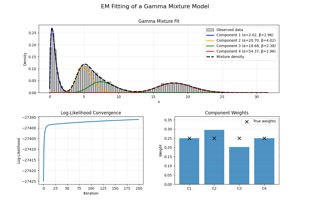
Conclusion
To summerize, we must say that fitting a mixture of Gamma is not much harder than fitting a Gaussian one, the EM structure is identical and the on ly difference is in the M-step when looking for the new shape. A mixture of Gamma is the right tool for a large class of real world data that Gaussian components simply can’t describe honestly. Here are some key ideas to take away from this post:
- Gamma mixtures are a powerful tool for modeling delays, durations, intensities, financial quantities, reliability measurements, and many stochastic processes where positivity and skewness are fundamental properties of the data.
- The EM algorithm can be adapted to fit Gamma mixtures and it’s the same recipe as for Gaussian mixtures.
- As always, initialization is important for EM, using k-means to initialize the parameters is a common practice.
- Choose the number of components wisely, you can use methods like BIC or AIC to help with that.
References
-
Bilmes, J. (1997). A Gentle Tutorial of the EM algorithm and its application to Parameter Estimation for Gaussian Mixture and Hidden Markov Models (Technical Report No. TR-97-021). International Computer Science Institute (ICSI). ↩ ↩2 ↩3
-
J. Almhana, Z. Liu, V. Choulakian and R. McGorman, “A Recursive Algorithm for Gamma Mixture Models,” 2006 IEEE International Conference on Communications, Istanbul, Turkey, 2006, pp. 197-202, doi: 10.1109/ICC.2006.254727. ↩